Microsoft Excel Tutorials - Home Page

Welcome to the World of Microsoft Excel - The Only Solution for all kinds of Business

Enter Microsoft Excel Tutorials

Here you will find Microsoft Excel 2003 tutorials, Microsoft Excel 2007 tutorials, Microsoft Excel Advanced Tutorials, Microsoft Excel tutorials using Macro, Microsoft Excel Tutorials using Visual Basic, Microsoft Excel Tutorials in high end, Microsoft Excel Tutorials for Quantity Surveyors, Microsoft Excel Tutorials for Planning Engineers, Microsoft Excel Software Free Download, Microsoft Excel Tutorials from Torrents, Microsoft Excel Video Tutorials, Microsoft Excel Tutorials e-books and a lot to come.. Watch this space for more... Microsoft Excel Macros Tutorials, Microsoft Excel VBA Programming.

Use the IF function to calculate the commissions for individual sales - Logical Functions - Microsoft Excel Tutorials

11.  Use the IF function to calculate the commissions for individual sales

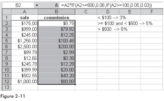
A company has a policy for individual commissions depending on sales, as shown below:
Sale < $100                                                3%
Sale => $100 and < $500                           5%
Sale >= $500                                              8%

To calculate the commissions:


1. Enter different possible sales amounts in column A.
2. Select cells B2:B12 and type the following formula: =A2*IF(A2>=500,0.08,IF(A2>=100,0.05,0.03)).
3. Press <-Ctrl+Enter->.

Watch the Video Tutorial - https://www.youtube.com/watch?v=UZYtm0IN5YM

 

Hope You Like This Tutorials - Give Comments

Combine IF with AND to check several conditions - Logical Functions - Microsoft Excel Tutorials

7.  Combine IF with AND to check several conditions:


In this example, Excel evaluates which condition meets the criteria and returns the result in the same row.

To combine the IF and AND functions:

1. Copy the content of cells C2 to C5 in Figure 2-7 to your Excel table.
2. Frame the table as shown in the screenshot
3. Select cell A2 and enter any kind of sales value, e.g., 120.
4. In cell B2, type the following formula: =IF(AND($A$2<=100,$A$2""),"Sales value is","").
5. In cell B3, type the following formula: =IF(AND($A$2>100,$A$2<=150)," Sales value is ","").
6. In cell B4, type the following formula: =IF(AND($A$2>150,$A$2<=200)," Sales value is ","").
7. In cell B5, type the following formula: =IF($A$2>200,"Sales value is ","").

Watch the Video Tutorial - https://www.youtube.com/watch?v=unjOBizKavM

  Hope You Like This Tutorials - Give Comments

Use the IF function to check for larger, equivalent, or smaller values - Logical Functions - Microsoft Excel Tutorials

6.  Use the IF function to check for larger, equivalent, or smaller values

In the previous example, two different messages were used as the result for comparing values. To check for three conditions in column A and present the result as “Column A is larger,” “equal,” or “Column A is smaller,” perform the following steps.

To compare columns and show the result:

1. Copy the previous example.
2. Select cells C2:C12 and type the following formula: =IF(A2>B2,"Column A is larger",IF(A2=B2,"equal",
"Column A is smaller")).
3. Press <-Ctrl+Enter->.

Note: Up to seven IF functions can be combined in one cell.  To combine more than seven functions, use the customized  solution near the end of this chapter.



Watch the Video Tutorial - https://www.youtube.com/watch?v=CbmCL1OvC88

Hope You Like This Tutorials, Give Comments

Use the IF function to compare columns and return a specific result - Logical Functions - Microsoft Excel Tutorials

5.  Use the IF function to compare columns and return a specific result

As shown in earlier examples, Excel returns the value TRUE or FALSE when using the OR and AND functions. The IF function can also be used to conduct conditional tests on values and formulas.

This example compares two columns and shows the result in column C.

To return specific text after comparing values:

1. Enter in range A2:A12 values from 1 to 1000.
2. Enter in range B2:B12 values from 1 to 1000.
3. Select cells C2:C12 and type the following formula: =IF(A2>=B2,"Column A is greater or equal","Column B is greater").
4. Press <-Ctrl+Enter->.

Watch the Video Tutorial - https://www.youtube.com/watch?v=DrkI_VS6l1Y

Hope You Like This Tutorial - Give Comments

Use the OR function to check cells for numbers - Logical Functions - Microsoft Excel Tutorials

4.  Use the OR function to check cells for numbers

A worksheet contains several values in column A. Each row has to be evaluated based on certain criteria in column A. The OR function is used for this task. The function returns TRUE if any argument is TRUE and FALSE if all arguments are FALSE.

Note: Up to 30 conditions can be used in one formula.

To check for two or more criteria:

1. Enter in range A2:A12 values from –43 to 100.
2. Select cells B2:B12 and type the following formula: =OR(A2=1,A2>=99,A2<0).
3. Press <-Ctrl+Enter->.

Watch the Video Tutorial - https://www.youtube.com/watch?v=LOanWoCrxKM

  Hope You Like This Tutorial - Give Comments

Use the OR function to check cells for text - Logical Functions - Microsoft Excel Tutorials

3.  Use the OR function to check cells for text

A worksheet contains several words in column A. Each row has to be checked for the words “new” or “actual” in column A. The OR function is used for this task. The function returns TRUE if either argument is true and FALSE if the arguments are not true.

Note: Up to 30 conditions can be used in one formula.

To use the OR function to check for two or more criteria:

1. Enter in range A2:A11 words like “new,” “actual,” and “old.”
2. Select cells B2:B11 and type the following formula: =OR(A2="New",A2="actual").
3. Press <-Ctrl+Enter->.

Watch the Video Tutorial - https://www.youtube.com/watch?v=dgoemyel0fw

  Hope You Like This Tutorial - Give Comments

Use the AND function to show sales for a specific period of time - Logical Functions - Microsoft Excel Tutorials

2.  Use the AND function to show sales for a specific period of time

This example checks all rows for a specific time period using the AND function. The function returns TRUE if the arguments are TRUE and FALSE if one or more arguments are FALSE.

Note: Up to 30 conditions can be used in one formula.

To show sales in a period of time:

1. Select cell B1 and enter the start date.
2. Select cell B2 and enter the end date.
3. The range A5:A16 contains dates from 09/13/04 to 09/21/04.
4. The range B5:B16 contains sales amounts.
5. Select cells C5:C16 and type the following formula: =AND(A5>=$B$1,A5<=$B$2).
6. Press <-Ctrl+Enter->.

Watch the Video Tutorial - https://www.youtube.com/watch?v=3jsUMabKeGY

  Hope You Like This Tutorial - Give Comments

Use the AND function to compare two columns - Logical Functions - Microsoft Excel Tutorials

Use the AND function to compare two columns

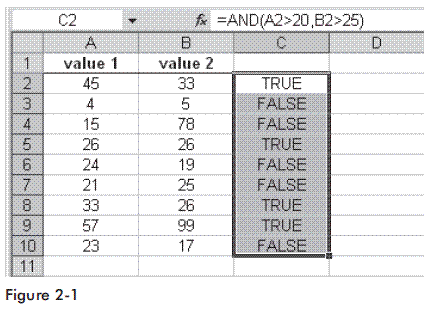
Two columns in a worksheet have to be evaluated. If the value in column A is greater than 20 and the value in column B is greater than 25, both values are valid.

To compare two columns:

1. In cells A2:A10, enter values from 1 to 100.
2. In cells B2:B10, enter values from 1 to 100.
3. Select cells C2:C10 and type the following formula: =AND(A2>20,B2>25).
4. Press <-Ctrl+Enter->.

Note: If both criteria are valid, Excel shows the value as TRUE; otherwise it is FALSE.




Watch the Video Tutorial - https://www.youtube.com/watch?v=CG4gircKYs0

  Hope You Like This Tutorial - Give Comments

Calculate the average speed - Formulas In Excel - Microsoft Excel Tutorials

36.  Calculate the average speed

In this example, someone travels from New York to Los Angeles with an average speed of 90 miles per hour. On the way back, the average speed is 75 miles per hour. What is the overall average speed?

To calculate the average speed, the speed in each direction has to be taken into consideration.

To calculate the overall average speed:

1. In cell C2, enter 90.
2. In cell C3, enter 75.
3. In cell C4, type the following formula: =(C2+C3)/2.

Watch the Video Tutorial - https://www.youtube.com/watch?v=NiSfJAtMSfg

  Hope You Like This Tutorial - Give Comments

Dividing and doubling every three hours - Formulas In Excel - Microsoft Excel Tutorials

35.  Dividing and doubling every three hours

In an experiment bacteria divides and doubles every three hours. How many bacteria will there be at the end of one day (24 hours)?

To calculate the total amount of bacteria after 24 hours:

1. Enter values from 1 to 4 in cells B2:B8.
2. Select cells C2:C8 and type the following formula: =A2^(24/B2).
3. Press <-Ctrl+Enter->.
4. From the Format menu, select Cells and the Number tab.
5. Choose Number from Category.
6. Set Decimal places to 0, and click on the Use 1000 Seperator check box.
7. Click OK.

Note: To insert the ^ character, press the <-^-> key on the keyboard followed by a <-Space->.

Watch the Video Tutorial - https://www.youtube.com/watch?v=VabcC1DmI6s

  Hope You Like This Tutorial - Give Comments

Calculate percentage of price reduction - Formulas In Excel - Microsoft Excel Tutorials

34.  Calculate percentage of price reduction

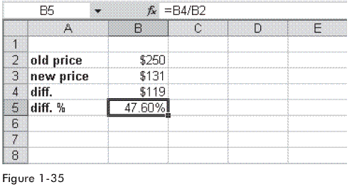
A digital camera is on sale. The camera’s original price is $250, but it is now available for $131. What is the percentage of the reduction?

To calculate the price reduction as a percentage:

1. Select cell B2 and enter the original price: $250.
2. In cell B3, enter the sales price: $131.
3. Calculate the absolute difference in cell B4 with the formula =B2-B3.
4. Determine the percentage of price reduction in cell B5 using the following formula: =B4/B2.
5. From the Format menu, select Cells.
6. Select the Number tab and click the category Percentage.
7. Click OK.

Watch the Video Tutorial - https://www.youtube.com/watch?v=tqcZA2rVvkk

  Hope You Like This Tutorial - Give Comments

Calculate Your Net Income - Formulas In Excel - Microsoft Excel Tutorials

33.  Calculate your net income

People often talk about their gross income. To calculate net income, it is necessary to consider the tax percentage using the following calculation.

To calculate net income:

1. Select cell B1 and enter the tax as a percentage: 33%.
2. In cell B2, enter the gross income: $3500.
3. Select cell B3 and type the formula =B2*B1 to calculate the tax amount.
4. Determine the net income in cell B4 with the formula =B2-B3.

Note: The amounts in cells B1 and B2 can be changed.



Watch the Video Tutorial - https://www.youtube.com/watch?v=u9L8ean6qK8

Hope You Like This Tutorial - Give Comments

Distribute sales - Formulas In Excel - Microsoft Excel Tutorials

32.  Distribute sales

In a company each sale is assigned to a particular salesperson. The sale of 30 pieces totals $199,000. Each salesperson sold an individual amount of goods. Calculate the corresponding sales for each person.

To calculate the total amount of sales for each employee:

1. Select cell B1 and enter the total amount of sales: 199000.
2. Select cell C1 and enter the total amount of sold goods: 30.
3. In columns A and B, enter the names of the salespeople and the number of pieces they sold.
4. Select cells C5:C11 and type the following formula: =B5*$B$1/$B$2.
5. Press <-Ctrl+Enter->.

Note: Check out the AutoSum of the selected range in the status bar.

Watch the Video Tutorial - https://www.youtube.com/watch?v=wORM9IycFB4

  Hope You Like This Tutorial - Give Comments

Calculate manpower required for a project - Formulas In Excel - Microsoft Excel Tutorials

31.  Calculate manpower required for a project

The number of employees needed for a project has to be calculated. To do this, enter the available time (14 days) for the project in cell A2. Cell B2 contains the number of working hours per day (8.5). Cell C2 shows the current number of employees. Now we can calculate how many employees are needed to reduce the project duration or change the number of daily working hours of the employees.

To calculate the desired number of employees:

1. Enter different combinations of desired days in column A and daily working hours in column B.
2. Select cell E2 and insert the formula =A2*B2*C2 to calculate the total working hours of the project.

3. Select cells C4:C9 and type the following formula: =ROUNDUP(C$2*A$2*B$2/(A4*B4),0).

4. Press <-Ctrl+Enter->.
5. Select cells E4:E9 and type the following formula: =A4*B4*C4.
6. Press <-Ctrl+Enter->.

Watch the Video Tutorial - https://www.youtube.com/watch?v=k3V8Ucovm6E

  Hope You Like This Tutorial - Give Comments

Determine how many pieces to put in a box - Formulas In Excel - Microsoft Excel Tutorials

30.  Determine how many pieces to put in a box

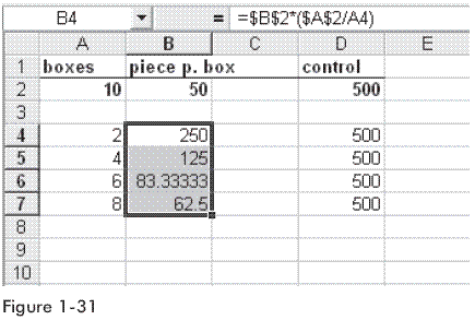
Let’s say a container can hold 10 boxes and each box can hold up to 300 items. The customer requires a total of 500 items. How many items must be packed in each box, given a number of boxes?

To determine the number of pieces in each box:

1. Select cell A2 and enter 10.
2. Select cell B2 and enter 50.
3. Select cell D2 and type =B2*A2.
4. In cells A4:A7 enter the number of boxes from 2 to 9.
5. Select cells B4:B7 and type the following formula: =$B$2*($A$2/A4).
6. Press <-Ctrl+Enter->.
7. Select cells D4:D7 and type the formula =B4*A4.
8. Press <-Ctrl+Enter->.

Note: Some entries in column A may result in a number with a decimal point in column B. These will require
additional calculation on your part to determine exactly how many pieces fit in the given number of boxes so that the customer receives exactly 500 pieces.



Watch the Video Tutorial - https://www.youtube.com/watch?v=XswP5CJWc3s

  Hope You Like This Tutorial - Give Comments

Determine the price per pound - Formulas In Excel - Microsoft Excel Tutorials

29.  Determine the price per pound

A worksheet lists food products in column A. Column B shows the corresponding weight in pounds, and column C contains the total price. What is the price per pound?

To calculate the price per pound:

1. In a workshop, enter the data shown in Figure 1-30, or use your own data.
2. Select cells D2:D8.
3. Type the following formula: =C2/B2.
4. Press <-Ctrl+Enter->.

Watch the Video Tutorial - https://www.youtube.com/watch?v=JEQzo0UUIgs

  Hope You Like This Tutorial - Give Comments

Calculate number of hours between two dates - Formulas In Excel - Microsoft Excel Tutorials

28.  Calculate number of hours between two dates

Excel has a problem calculating the difference between two dates in hours. Try this by opening a new worksheet and typing the starting date including time (3/20/2006 13:42) in cell A2. In cell B2, type the end date and time (3/24/2006 7:42). Then subtract B2 from A2 in cell C2. The calculation generates 1/3/1900 18:00, which is incorrect. If your result displays #####, you’ll need to extend the width of column C.

To properly format the difference in hours:

1. Select cell C2.
2. From the Format menu, select Cells and choose the Number tab.
3. Select Custom from Category.
4. Type the custom format [hh]:mm.

5. Click OK. This gives the correct answer.

Watch the Video Tutorial - https://www.youtube.com/watch?v=ItvfCf5QNMg

  Hope You Like This Tutorial - Give Comments

Monitor the daily production plan (Productivity Calculation) - Formulas In Excel - Microsoft Excel Tutorials

27.  Monitor the daily production plan

A worksheet is used to monitor daily production. The target is defined as 1,500 pieces per day. To calculate the percentage produced of the daily goal, perform the following steps.

To monitor daily production:

1. Select cell B1 and enter the predefined target: 1500.
2. Select cells C4:C11 and type the following formula: =B4/$B$1.
3. Press <-Ctrl+Enter->.
4. From the Format menu, select Cells and the Number tab.
5. Choose Percentage from Category.
6. Set Decimal places to 2.
7. Click OK.

Watch the Video Tutorial - https://www.youtube.com/watch?v=Y2D6n7BrbbY

  Hope You Like This Tutorial - Give Comments

Calculation with percentage of completion - Formulas In Excel - Microsoft Excel Tutorials

26.  Calculation with percentage

Let’s say you want to buy a new car. The listed price of the car is $25,500, and the tax to be added is 8%. After negotiating a sales discount of 10%, the final price has to be calculated.

To calculate the final price:

1. Select cell B1 and enter 25500.
2. Select cell B2 to enter the tax rate of 8%.
3. Select cell B3 and enter the discount rate of 10%.
4. Select cell B5 and type the following formula: =B1*(1+B2)*(1-B3).

Note: As you see in cell C5 in Figure 1-26, the formula =B1*(1–B3)*(1+B2) also works. The order of multiplication does not matter.

Watch the Video Tutorial - https://www.youtube.com/watch?v=efqUK_onU7c

 

Hope You Like This Tutorial - Give Comments