Use the IF function to create your own timesheet - Logical Functions - Microsoft Excel Tutorials

17.  Use the IF function to create your own timesheet

In the last example for this chapter we create our own timesheet, step by step. First, press <-Shift+F11-> to insert a new worksheet.  Then create the following timesheet as an example:

We have to consider that the daily target of eight hours is still fulfilled when an employee is ill (IL), on holiday (HO), or in training (TR). For other days, the number of working hours has to be calculated.

To calculate the daily working hours:

1. Select cell F2:F6 and type the following formula: =IF(OR(C2="TR",C2="IL",C2="HO"),E2,D2-C2).
2. Press <-Ctrl+Enter->.

Watch the Video Tutorial - https://www.youtube.com/watch?v=kAAoVojjaNc

  Hope You Like This Tutorial - Give Comments

Use the IF function combined in one cell more than seven times - Logical Functions - Microsoft Excel Tutorials

15.  Use the IF function combined in one cell more than seven times

The Excel online help says that it is not possible to combine the IF function more than seven times. That is not true, as shown below.

To insert more than seven conditions:

1. Select cell A1 and enter 12.
2. Select cell B1 and type the following formula:

=IF(A2=1,A2,IF(A2=2,A2*2,IF(A2=3,A2*3,IF(A2=4 ,A2*4,IF(A2=5,A2*5,IF(A2=6,A2*6,IF(A2=7,A2*7,)))))))+IF(A2=8,A2*8,IF(A2=9,A2*9,IF(A2=10,A2*10,)))+IF(A2=11,A2*11,IF(A2=12,A2*12,)).

3. Press <-Enter->.

Watch the Video Tutorial - https://www.youtube.com/watch?v=cr3yOPVMsYw

  Hope You Like This Tutorial - Give Comments

Use the TYPE function to check for invalid values - Logical Functions - Microsoft Excel Tutorials

14.  Use the TYPE function to check for invalid values

Sometimes Excel cannot interpret some values, especially imported data. As an example, let’s say a cell contains an apparent value but the calculation leads to an incorrect result. To prevent this, use the IF function in combination with TYPE to check for invalid data in the worksheet. This example will enter the text “invalid value” in column B if the value entered in column A is not numeric.

To show invalid values in a worksheet:



1. Enter some values or text in column A.
2. Select cells B2:B10 and type the following formula: =IF(AND(TYPE(A2)=1,A2""),A2,"invalid value").
3. Press <-Ctrl+Enter->.

Watch the Video Tutorial - https://www.youtube.com/watch?v=0aN7FEbYJq4

  Hope You Like This Tutorial - Give Comments

Use the INT function with the IF function - Logical Functions - Microsoft Excel Tutorials

13.  Use the INT function with the IF function


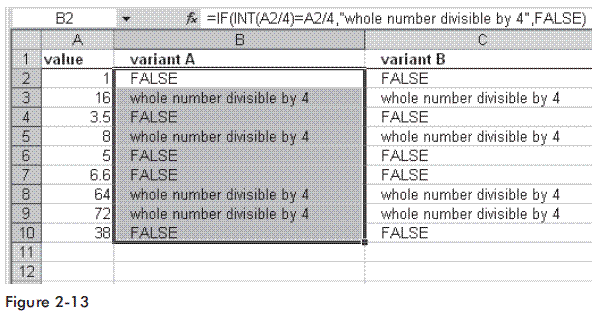
To see if one value is a whole number and can be divided by another value, use the IF function in combination with the INT function.

To see if a whole number can be divided by 4:

1. Select cells B2:B10 and type the following formula: =IF(INT(A2/4)=A2/4,"whole number divisible by 4",FALSE).
2. Press <-Ctrl+Enter->.

Or

1. Select cells C2:C10 and type the following formula: =IF(A2/4-INT(A2/4)=0,"whole number divisible by 4", FALSE).
2. Press <-Ctrl+Enter->.

Watch the Video Tutorial - https://www.youtube.com/watch?v=9uIAT7uGFXQ

  Hope You Like This Tutorials - Give Comments

Use the IF function to compare two cells - Logical Functions - Microsoft Excel Tutorials

12.  Use the IF function to compare two cells


The following tip is a solution for comparing two cells line by line.  Prepare a new worksheet, filling the first two columns with the values 0 and 1 as shown in Figure 2-12.


To compare cells line by line:


1. Select cells C2:C11 and type the following formula: =IF(A2&B2="11","OK",IF(A2&B2="10","First Value is OK",IF(A2&B2="01","Second Value is OK",”Both Values are FALSE”))).
2. Press <-Ctrl+Enter->.

Watch the Video Tutorial - https://www.youtube.com/watch?v=vHIrcO8B0gM

Hope You Like This Tutorials - Give Comments

Use the IF function to calculate the commissions for individual sales - Logical Functions - Microsoft Excel Tutorials

11.  Use the IF function to calculate the commissions for individual sales

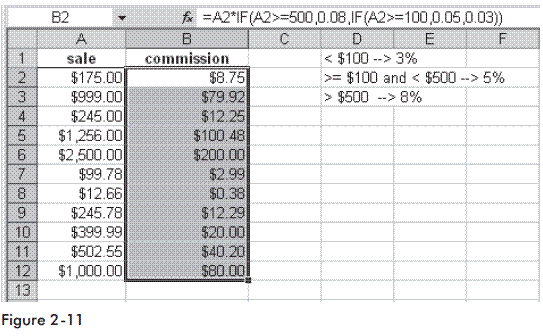
A company has a policy for individual commissions depending on sales, as shown below:
Sale < $100                                                3%
Sale => $100 and < $500                           5%
Sale >= $500                                              8%

To calculate the commissions:


1. Enter different possible sales amounts in column A.
2. Select cells B2:B12 and type the following formula: =A2*IF(A2>=500,0.08,IF(A2>=100,0.05,0.03)).
3. Press <-Ctrl+Enter->.

Watch the Video Tutorial - https://www.youtube.com/watch?v=UZYtm0IN5YM

 

Hope You Like This Tutorials - Give Comments

Use the IF function to check cells in worksheets and workbooks - Logical Functions - Microsoft Excel Tutorials

9.  Use the IF function to check cells in worksheets and workbooks

To use an IF statement not only in a worksheet but also in a linked worksheet or workbook, start typing part of the formula, for example, “ =IF(,” then navigate to another worksheet or open up a workbook, select the desired cell, and go back to the first worksheet to finish the formula.

To use the IF function to check out cells in another worksheet:

Type =IF(Sheet8!A2"january","wrong month","OK").

To use the IF function to check out cells in another workbook:

Type =IF('C:\Held\Formulas\Files\[Formulas.xls]Sheet35'!$A$1<>1,"wrong","OK").

Watch the Video Tutorial - https://www.youtube.com/watch?v=1tTcyhSnXzU

Hope You Like This Tutorials - Give Comments

Use the IF function to determine the quarter of a year - Logical Functions - Microsoft Excel Tutorials

8.  Use the IF function to determine the quarter of a year

After entering an initial value, Excel can automatically fill worksheet cells with the names of weekdays or months. Open a new worksheet and type the word “January” in cell A2. Then drag the lower-right point of this cell down to A13 to let Excel create a list containing the months of the year. In this example, we want to indicate which months fall into which quarter.

To determine the quarter of a year in which a particular month falls:


1. Select cells B2:B13 and type the following formula: =IF(OR(A2="January",A2="February",A2="March"),"1st quarter",IF(OR(A2="April",A2="May",A2="June"),"2nd quarter",IF(OR(A2="July",A2="August",A2="September"),"3rd quarter","4th quarter"))).
2. Press <-Ctrl+Enter->.

Watch the Video Tutorial - https://www.youtube.com/watch?v=y8W05VSN0r0

Hope You Like TTutorials - Give Comments

Combine IF with AND to check several conditions - Logical Functions - Microsoft Excel Tutorials

7.  Combine IF with AND to check several conditions:


In this example, Excel evaluates which condition meets the criteria and returns the result in the same row.

To combine the IF and AND functions:

1. Copy the content of cells C2 to C5 in Figure 2-7 to your Excel table.
2. Frame the table as shown in the screenshot
3. Select cell A2 and enter any kind of sales value, e.g., 120.
4. In cell B2, type the following formula: =IF(AND($A$2<=100,$A$2""),"Sales value is","").
5. In cell B3, type the following formula: =IF(AND($A$2>100,$A$2<=150)," Sales value is ","").
6. In cell B4, type the following formula: =IF(AND($A$2>150,$A$2<=200)," Sales value is ","").
7. In cell B5, type the following formula: =IF($A$2>200,"Sales value is ","").

Watch the Video Tutorial - https://www.youtube.com/watch?v=unjOBizKavM

  Hope You Like This Tutorials - Give Comments

Use the IF function to check for larger, equivalent, or smaller values - Logical Functions - Microsoft Excel Tutorials

6.  Use the IF function to check for larger, equivalent, or smaller values

In the previous example, two different messages were used as the result for comparing values. To check for three conditions in column A and present the result as “Column A is larger,” “equal,” or “Column A is smaller,” perform the following steps.

To compare columns and show the result:

1. Copy the previous example.
2. Select cells C2:C12 and type the following formula: =IF(A2>B2,"Column A is larger",IF(A2=B2,"equal",
"Column A is smaller")).
3. Press <-Ctrl+Enter->.

Note: Up to seven IF functions can be combined in one cell.  To combine more than seven functions, use the customized  solution near the end of this chapter.



Watch the Video Tutorial - https://www.youtube.com/watch?v=CbmCL1OvC88

Hope You Like This Tutorials, Give Comments

Use the IF function to compare columns and return a specific result - Logical Functions - Microsoft Excel Tutorials

5.  Use the IF function to compare columns and return a specific result

As shown in earlier examples, Excel returns the value TRUE or FALSE when using the OR and AND functions. The IF function can also be used to conduct conditional tests on values and formulas.

This example compares two columns and shows the result in column C.

To return specific text after comparing values:

1. Enter in range A2:A12 values from 1 to 1000.
2. Enter in range B2:B12 values from 1 to 1000.
3. Select cells C2:C12 and type the following formula: =IF(A2>=B2,"Column A is greater or equal","Column B is greater").
4. Press <-Ctrl+Enter->.

Watch the Video Tutorial - https://www.youtube.com/watch?v=DrkI_VS6l1Y

Hope You Like This Tutorial - Give Comments

Use the OR function to check cells for numbers - Logical Functions - Microsoft Excel Tutorials

4.  Use the OR function to check cells for numbers

A worksheet contains several values in column A. Each row has to be evaluated based on certain criteria in column A. The OR function is used for this task. The function returns TRUE if any argument is TRUE and FALSE if all arguments are FALSE.

Note: Up to 30 conditions can be used in one formula.

To check for two or more criteria:

1. Enter in range A2:A12 values from –43 to 100.
2. Select cells B2:B12 and type the following formula: =OR(A2=1,A2>=99,A2<0).
3. Press <-Ctrl+Enter->.

Watch the Video Tutorial - https://www.youtube.com/watch?v=LOanWoCrxKM

  Hope You Like This Tutorial - Give Comments

Use the OR function to check cells for text - Logical Functions - Microsoft Excel Tutorials

3.  Use the OR function to check cells for text

A worksheet contains several words in column A. Each row has to be checked for the words “new” or “actual” in column A. The OR function is used for this task. The function returns TRUE if either argument is true and FALSE if the arguments are not true.

Note: Up to 30 conditions can be used in one formula.

To use the OR function to check for two or more criteria:

1. Enter in range A2:A11 words like “new,” “actual,” and “old.”
2. Select cells B2:B11 and type the following formula: =OR(A2="New",A2="actual").
3. Press <-Ctrl+Enter->.

Watch the Video Tutorial - https://www.youtube.com/watch?v=dgoemyel0fw

  Hope You Like This Tutorial - Give Comments

Use the AND function to show sales for a specific period of time - Logical Functions - Microsoft Excel Tutorials

2.  Use the AND function to show sales for a specific period of time

This example checks all rows for a specific time period using the AND function. The function returns TRUE if the arguments are TRUE and FALSE if one or more arguments are FALSE.

Note: Up to 30 conditions can be used in one formula.

To show sales in a period of time:

1. Select cell B1 and enter the start date.
2. Select cell B2 and enter the end date.
3. The range A5:A16 contains dates from 09/13/04 to 09/21/04.
4. The range B5:B16 contains sales amounts.
5. Select cells C5:C16 and type the following formula: =AND(A5>=$B$1,A5<=$B$2).
6. Press <-Ctrl+Enter->.

Watch the Video Tutorial - https://www.youtube.com/watch?v=3jsUMabKeGY

  Hope You Like This Tutorial - Give Comments

Use the AND function to compare two columns - Logical Functions - Microsoft Excel Tutorials

Use the AND function to compare two columns

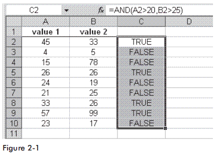
Two columns in a worksheet have to be evaluated. If the value in column A is greater than 20 and the value in column B is greater than 25, both values are valid.

To compare two columns:

1. In cells A2:A10, enter values from 1 to 100.
2. In cells B2:B10, enter values from 1 to 100.
3. Select cells C2:C10 and type the following formula: =AND(A2>20,B2>25).
4. Press <-Ctrl+Enter->.

Note: If both criteria are valid, Excel shows the value as TRUE; otherwise it is FALSE.




Watch the Video Tutorial - https://www.youtube.com/watch?v=CG4gircKYs0

  Hope You Like This Tutorial - Give Comments