Use the SUM function to sum a range - Mathematical Functions - Microsoft Excel Tutorials

Use the SUM function to sum a range using Microsoft Excel

In this example, each value of a range in a worksheet has to be added, with the sum appearing in cell A11. To do this, use the SUM function, which returns the sum of all numbers in a range of cells.

SUM(number1, number2, ...)

number1, number2, ...: From 1 to 30 arguments to be summed up. Cell references are also valid.

To sum a range:

1. In cells A2:A10 enter any values from 1 to 100. Figure shows that we used dollar amounts.
2. In cell A11 type the following formula: =SUM(A1:A10).
3. Press <-Enter->.

Use the SUM function to sum a range

Note: To perform this task a little faster, just select cell A11 and click on the icon (AutoSum) on the Standard toolbar. Then press <-Enter-> to display the result of the calculation.

Use the STDEV function to determine the standard deviation - Basic Statistical Functions - Microsoft Excel Tutorials

Use the STDEV function to determine the standard deviation using Microsoft Excel

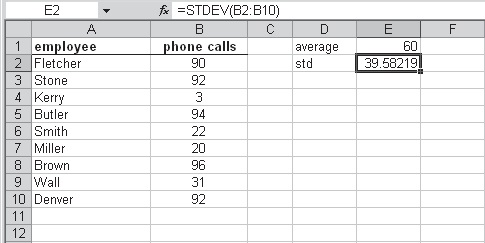
In this example, the standard deviation of the number of phone calls has to be determined. Use the STDEV function for this purpose. This function measures how widely values in a set differ from the average, or mean, value.

STDEV(number1, number2, ...)

number1, number2, ...: From 1 to 30 numerical arguments that represent a population sample.

To determine the standard deviation for employee phone calls:

1. In cells A2:A10 type the names of your employees.
2. In cells B2:B10 type the number of phone calls the employees make per month.
3. Select cells E2 and type the following formula: =STDEV(B2:B10).
4. Press <-Enter->.

Use the STDEV function to determine the standard deviation

Use the QUARTILE function to calculate the quartiles - Basic Statistical Functions - Microsoft Excel Tutorials

Use the QUARTILE function to calculate the quartiles using Microsoft Excel

In this example, the quartile of a list has to be determined. The QUARTILE function returns the quartile of a data set. Quartiles are used to divide populations into four classes with each containing one-fourth of the total population.

QUARTILE(array, quart)

array: An array or cell range of numeric values for which you want to find the quartile value.

quart: A number from 0 to 4 that specifies the value to return. (0 = Minimum value, 1 = First quartile (25th percentile), 2 = Median value (50th percentile), 3 = Third quartile (75th percentile), 4 = Maximum value)

To determine the quartiles into which employee telephone use falls:

1. In cells A2:A10 type the names of your employees.
2. In cells B2:B10 type the number of phone calls the employees make per month.
3. Select cells D2 and type the following formula: =QUARTILE($B$2:$B$10,0).
4. Select cells D3 and type the following formula: =QUARTILE($B$2:$B$10,1).

Use the QUARTILE function to calculate the quartiles

Use the MEDIAN function to calculate the median sales - Basic Statistical Function - Microsoft Excel Tutorials

Use the MEDIAN function to calculate the median sales using Microsoft Excel

In this example the average and median sales for a month have to be determined. Use the data shown in Figure and calculate the average sales in cell E2. To calculate the median of the sales, use the MEDIAN function. The median is a value in the middle of a set of values; that is, half the values are above the median and half the values are below.

MEDIAN(number1, number2, ...)

number1, number2,… : From 1 to 30 numbers for which you want to find the median.

To calculate the median sales:

1. In cells A2:A13 type the month.
2. In cells B2:B13 type the monthly sales.
3. Select cells E1 and type the following formula: =MEDIAN(B2:B13).
4. Press <-Enter->.

Use the MEDIAN function to calculate the median sales

Note: You can find the average, as shown in cell E2, by using the formula =AVERAGE(B2:B13).

Use the RANK function to determine the rank of sales - Basic Statistical Functions - Microsoft Excel Tutorials

Use the RANK function to determine the rank of sales using Microsoft Excel

To compare sales of several days and rank them, use the RANK function. This function returns a number that is the rank of a value. In this example, the list can be sorted to display sales in rank order.

RANK(number, ref, order)

number: The number for which we want to find the rank.
ref: A reference to a list of numbers. Only numeric values are considered.

order: A number that specifies the ranking method. If order is 0 or omitted, the numbers are ranked in descending order. If order is a nonzero value, the numbers are ranked in ascending order.

To rank a list in descending order:

1. In cells A2:A10 enter dates.
2. In cells B2:B10 enter the sales for each date.
3. Select cells C2:C10 and type the following formula: =RANK(B2,$B$2:$B$10).
4. Press <-Ctrl+Enter->.

Use the RANK function to determine the rank of sales

Note: If you want to rank in ascending order, use this formula: =RANK(B2,$B$2:$B$10,1).

Use the SUBTOTAL function to count rows in filtered lists - Basic Statistical Functions - Microsoft Excel Tutorials

Use the SUBTOTAL function to count rows in filtered lists using Microsoft Excel

When using the Filter option in the Data menu, it is recommended that the COUNT and COUNTA functions not be used because in a filtered worksheet they count both visible and hidden rows. Instead, use the SUBTOTAL function to get the subtotal of a list or database that is visible. The syntax for the SUBTOTAL function was presented earlier.

To count rows in a filtered list:

1. In cells B2:B10 type group numbers from 1 to 3.
2. In cells C2:C10 type the daily sales of each group.
3. From the Data menu, select Filter | AutoFilter.
4. Select group 1 in the column B filter.
5. Select cell C12 and type the following formula: =SUBTOTAL(2,C2:C10) & " rows in filter".

Use the SUBTOTAL function to count rows in filtered lists

Note: Use the function =SUBTOTAL(3,B2:B10) & " rows in filter" in cell B12 to count the filtered cells as seen in Figure

Use the COUNTA function to determine the last filled row - Basic Statistical Functions - Microsoft Excel Tutorials

Use the COUNTA function to determine the last filled row using Microsoft Excel

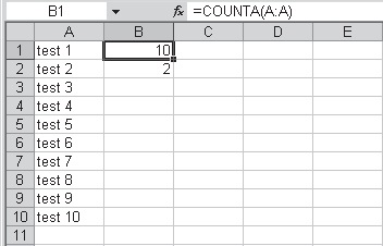
In this example, the last row that was filled in on a worksheet needs to be determined. If all cells of a column contain data and are not empty, the COUNTA function can be used. Define as the range the entire column in order to count all filled cells.

To determine the last filled row:

1. In cells A1:A10 type data (numeric and text).
2. Select cell B1 and type the following formula: =COUNTA(A:A).
3. Press <-Enter->.

Note: To determine the last column of a worksheet that was filled, use the function =COUNTA(1:1) as shown in cell B2.

Use the COUNTA function to determine the last filled row

Use the COUNTBLANK function to count empty cells - Basic Statistical Functions - Microsoft Excel Tutorials

Use the COUNTBLANK function to count empty cells using Microsoft Excel

Occasionally it is may be useful to determine how many cells in a range are empty. You can use the COUNTBLANK function to count all empty cells in a range of cells.

COUNTBLANK(range)

range: The range in which to count blank cells.

To count all empty cells in a specified range:

1. In cells A1:A10 type data (numeric and text). Be sure to leave a few cells empty.
2. Select cell C1 and type the following formula: =COUNTBLANK(A1:A10).
3. Press <-Enter->.

Use the COUNTBLANK function to count empty cells

Use the COUNTA function to count cells containing text - Basic Statistical Functions - Microsoft Excel Tutorials

Use the COUNTA function to count cells containing text using Microsoft Excel

To count all cells that contain text data, use a combination of functions in one formula. The number of cells with any kind of data is counted with the COUNTA function. All numeric cells are counted with the COUNT function. Just subtract the results of the COUNT function from the results of the COUNTA function, using the same range, to get all cells containing text.

To count only cells with text:

1. In cells A1:A10 type any kind of data (numeric and text).
2. Select cell C1 and type the following formula: =COUNTA(A1:A10)-COUNT(A1:A10).
3. Press <-Enter->.

Use the COUNTA function to count cells containing text

Use the COUNTA function to count cells containing data - Basic Statistical Functions - Microsoft Excel Tutorials

Use the COUNTA function to count cells containing data using Microsoft Excel

To count all cells that are not empty and contain data in a range or array, use the COUNTA function.

COUNTA(value1, value2, ...)

value1, value2, ...: 1 to 30 arguments representing the values to be counted.

To count all cells containing data:

1. In cells A1:A10 type any kind of data (numeric and text).
2. Select cell C1 and type the following formula: =COUNTA(A1:A10).
3. Press <-Enter->.

Use the COUNTA function to count cells containing data

Note: The COUNTA function does not count empty cells.

Use the COUNT function to count cells containing numeric data - Basic Statistical Functions - Microsoft Excel Tutorials

Use the COUNT function to count cells containing numeric data using Microsoft Excel

To count all cells that contain numbers, use the COUNT function. Empty cells, logical values, text, and error values are ignored.

COUNT(value1, value2, ...)

value1, value2, ...: From 1 to 30 arguments of any type of data.  However, all but numeric data is ignored.

To count the number of cells that contain numbers:

1. In cells A1:A10 type data (numeric and text).
2. Select cell C1 and type the following formula: =COUNT(A1:A10).
3. Press <-Enter->.

Use the COUNT function to count cells containing numeric data

Note: Arguments that are date and time values are counted as numeric too.

Use the SUBTOTAL function to sum a filtered list - Basic Statistical Functions - Microsoft Excel Tutorials

Use the SUBTOTAL function to sum a filtered list using Microsoft Excel

When using the Filter option in the Data menu, it is not advisable to use the SUM function to sum up filtered rows because it sums up all rows, including those that are hidden. Instead, use the SUBTOTAL function to get the subtotal of a list or database that is visible.

SUBTOTAL(function_num, ref1, ref2, ...)

function_num: A number from 1 to 11 that specifies a particular function to use for calculating subtotals. (1 = AVERAGE, 2 = COUNT, 3 = COUNTA , 4 = MAX, 5 = MIN, 6 = PRODUCT, 7 = STDEV, 8 = STDEVP, 9 = SUM, 10 = VAR, and 11 = VARP)

ref1, ref2, ...: From 1 to 29 ranges or references for which a subtotal is desired.

To sum a filtered list:

1. In cells B2:B10 type group numbers from 1 to 3.
2. In cells C2:C10 type the daily sales for each group.
3. From the Data menu, select Filter | AutoFilter.
4. Select group 1 in the column B filter.
5. Select cell C12 and type the following formula: =SUBTOTAL(9,C2:C10).

Use the SUBTOTAL function to sum a filtered list

Use the AVERAGE function to calculate the average output - Basic Statistical Functions - Microsoft Excel Tutorials

Use the AVERAGE function to calculate the average output using Microsoft Excel

In this example, the output of three production lines has been recorded for several days. Now the average of the three highest outputs of each line has to be calculated. For this task, Excel provides the AVERAGE function, which returns the average, or arithmetic mean, of the arguments.

AVERAGE(number1, number2, ...)

number1, number2, ...: From 1 to 30 numeric arguments for which you want to determine the average. It is also possible to use a cell reference, as shown in this example.

To calculate the average of the three highest capacities of each production line:

1. In cells B2:D10 type the output of each machine.
2. Select cells B13:D13 and type the following formula: =AVERAGE(LARGE(B$2:B$10,1),LARGE(B$2:B$10,2),LARGE(B$2:B$10,3)).
3. Press <-Ctrl+Enter->.

Use the AVERAGE function to calculate the average output

Use the SMALL function to compare prices and select the cheapest offer - Basic Statistical Functions - Microsoft Excel Tutorials

Use the SMALL function to compare prices and select the cheapest offer using Microsoft Excel

A worksheet lists offers from different suppliers. To make a decision as to which is the best offer, the SMALL function can be used to check for the lowest price. As in the previous tip, you can use the INDEX and MATCH functions to get the names of the companies.

To find out the three cheapest offers and their supplier:

1. In cells B2:B10 enter the offers.
2. Number the cells C2:C4 with 1, 2, and 3.
3. Select cells D2:D4 and type the following formula: =INDEX($A$2:$A$10,MATCH(SMALL($B$2:$B$10,C2),$B$2:$B$10,0)).
4. Press <-Ctrl+Enter->.
5. Select cells E2:E4 and type the following formula: =SMALL($B$2:$B$10,C2).
6. Press <-Ctrl+Enter->.

Use the SMALL function to compare prices and select the cheapest offer

Use the INDEX, MATCH, and LARGE functions to determine and locate the best salesperson - Basic Statistical Function - Microsoft Excel Tutorials

Use the INDEX, MATCH, and LARGE functions to determine and locate the best salesperson using Microsoft Excel

As seen in the previous tips, it is easy to find out the highest value in a list. But how do you find the one person on a sales team who sold the most? And how do you find out how much ahead of the others he or she is?  Start with the LARGE function to determine the highest sale. Then use the INDEX and MATCH functions to retrieve the name of the employee.

To determine and locate the best employee:

1. In cells B2:B10 type the daily sales of the employees.
2. Select cell D3 and type the following formula: =INDEX($A$2:$A$10,MATCH(LARGE($B$2:$B$10,1),$B$2:$B$10,0)).
3. Press <-Enter->.
4. Select cell D6 and type the following formula: =LARGE($B$2:$B$10,1)-LARGE($B$2:$B$10,2).
5. Press <-Enter->.

Use the INDEX MATCH and LARGE functions to determine and locate the best salesperson

Use the LARGE function to find the highest values - Basic Statistical Functions - Microsoft Excel Tutorials

Use the LARGE function to find the highest values using Microsoft Excel

To determine the highest value in a list, we used the MAX function. To find out multiple high values of a range, the LARGE function can be used. This function returns the nth highest value in a set of data.

LARGE(array, n)

array: Array or range of numerical data in which we want to find the nth highest value.
n: The position from the highest in the array or range of data to return.

To determine the three highest values of a range:

1. In cells A2:C10 type any values from 0 to 99.
2. Number cells A12, A13, and A14 with 1, 2, and 3.
3. Select cells B12:D14 and type the following formula:=LARGE(B$2:B$10,$A12).
4. Press <-Ctrl+Enter->.

Use the LARGE function to find the highest values

Use the SMALL function to find the smallest values in a list - Basic Statistical Functions - Microsoft Excel Tutorials

Use the SMALL function to find the smallest values in a list using Microsoft Excel

To determine the smallest value in a list, we can use the MIN function.  However, the easiest way to find multiple small values of a range is by using the SMALL function. This function returns the nth smallest value in a set of data.

SMALL(array, n)

array: An array or range of numerical data in which you want to find the nth smallest value.
n: The position from the smallest in the array or range of data to return.

To determine the three smallest values of a range:

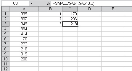
1. In cells A1:A10 enter any values from 100 to 999.
2. Select cell C1 and type the following formula =SMALL($A$1:$A$10,1) to get the smallest value.
3. In cell C2 type the formula =SMALL($A$1:$A$10,2) to get the second smallest value.
4. In cell C3 type the formula =SMALL($A$1:$A$10,3) to get the third smallest value.

Use the SMALL function to find the smallest values in a list

Use the MIN function to detect the smallest value in a column - Basic Statistical Functions - Microsoft Excel Tutorials

Use the MIN function to detect the smallest value in a column using Microsoft Excel

To determine the smallest value in a single column, the MIN function is used. This function returns the smallest value in a set of values. The syntax is described in the previous tip.

To determine the smallest value in a column:

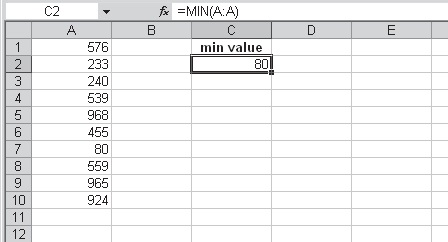
1. In column A, type any values down to cell A10.
2. Select cell B1 and type the following formula: =MIN(A:A).
3. Press <-Enter->.

Use the MIN function to detect the smallest value in a column

Note: To determine the smallest value in a row, such as the smallest value in the first row, use the formula =MIN(1:1). To get the smallest value of the first three rows, use the following function: =MIN(1:3).

Use the MIN function to find the employee with the lowest sales - Basic Statistical Functions - Microsoft Excel Tutorials

Use the MIN function to find the employee with the lowest sales using Microsoft Excel

In a company, employee sales are monitored. Columns B to E contain the sales for the first four months of the year. To determine which employee has the lowest monthly sales, use the MIN function. The function’s return value is the smallest value in a set.

MIN(number1, number2, ...)

number1, number2, ...: From 1 to 30 numbers for which you want to find the smallest value. It is possible to use a cell reference; however, the cells must contain numbers or values that can be converted to numbers.

To determine the lowest monthly sales:

1. In a worksheet, copy the range A1:E10 shown in Figure.
2. Select cells B12:E12 and type the following formula: =MIN(B2:B10).
3. Press <-Ctrl+Enter->.

Use the MIN function to find the employee with the lowest sales

Note: Later you will learn how to automatically shade the smallest value in each column.

Use the MAX function to determine the largest value in a range - Basic Statistical Functions - Microsoft Excel Tutorials

Use the MAX function to determine the largest value in a range using Microsoft Excel

This example finds the largest value in the range A3:D11 by using the MAX function. The function’s return value is the largest (Maximum) value in a set.

MAX(number1, number2, ...)

number1, number2, ...: From 1 to 30 numbers for which you want to find the largest value. It is possible to use a cell reference; however, the cells must contain numbers or values that can be converted to numbers.

To determine the largest value:

1. In cells A3:D11 type any values.
2. In cell B1 type the formula =MAX(A3:D11).
3. Press <-Enter->.

Use the MAX function to determine the largest value in a range

Note: Later you will learn how to automatically mark and shade the largest value in a range.