Use the TIME function to combine single time parts - Date and Time Functions - Microsoft Excel Tutorials

Use the TIME function to combine single time parts using Microsoft Excel

The worksheet in Figure 4-29 shows single time parts in each column. Column B contains hours, column C contains minutes, and column D contains seconds. All three columns have to be combined into one time as shown in column E. To do this, use the TIME function. This function returns the decimal number for a particular time. The syntax is:

TIME(hour, minute, second)

hour: A number from 0 to 23 that represents the hour. Any value greater than 23 will be divided by 24 and the remainder will be treated as the hour value.
minute: A number from 0 to 59 that represents minutes. Any value greater than 59 will be converted to hours and minutes.
second: A number from 0 to 59 that represents seconds. Any value greater than 59 will be converted to hours, minutes, and seconds.

To combine single time parts into a valid time:

1. Select cells E2:E10 and type the formula =TIME(B2,C2,D2).
2. Press <-Ctrl+Enter->.
3. From the Format menu, select Cells.
4. Select the Number tab and click Custom under Category.
5. Enter hh:mm:ss as the custom format.
6. Click OK.

Use the TIME function to combine single time parts

Use the HOUR function to calculate with 100-minute hours - Date and Time Functions - Microsoft Excel Tutorials

Use the HOUR function to calculate with 100-minute hours using Microsoft Excel

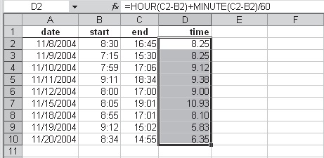
Some companies record working time in 100-minute hours. For example, the time 6:45 is converted to 6:75, which sometimes makes further calculations easier. To convert to this format, extract the minutes from the time and divide them by 60 using the MINUTE function. This function returns the minutes of a time value. The minute is given as an integer, ranging from 0 to 59. The hours can be extracted with the HOUR function. This function returns the hour of a time value as an integer ranging from 0 (12:00 a.m.) to 23 (11:00 p.m.).

To convert normal time to 100-minute hours:

1. In cells A2:A10 list work dates.
2. In cells B2:B10 enter the start time for each day.
3. In cells C2:C10 record the end times.
4. Select cells D2:D10 and type the following formula: =HOUR(C2-B2)+MINUTE(C2-B2)/60.
5. Press <-Ctrl+Enter->.

Use the HOUR function to calculate with 100-minute hours

Use a custom format to create a time format - Date and Time Functions - Microsoft Excel

Use a custom format to create a time format using Microsoft Excel

When you enter time values in cells, you have to type the colon between the hours and minutes. However, this is unnecessary if you use a custom format.

To create a customized time format:

1. Enter time values without colons and select the cells.
2. From the Format menu, select Cells.
3. Select the Number tab and click on Custom under Category.
4. Type 00":"00 as the custom format.
5. Click OK.

Use a custom format to create a time format

Note: You can also use the AutoCorrect options. From the Tools menu, choose AutoCorrect and then the AutoCorrect tab. Type two commas in the Replace field and type the colon in the With field. Click Add to insert this option. Test this by typing 1200 in a cell. Excel corrects the input to 12:00.

Use the TIMEVALUE function to convert text to time - Date and Time Functions - Microsoft Excel Tutorials

Use the TIMEVALUE function to convert text to time using Microsoft Excel

In this example, a text string has to be converted to a valid time. Columns A and C contain different start and end times as part of a standardized text string. It is possible to extract the times and convert them to valid time values that can be used as the basis for calculations. To convert text into a valid time, use the TIMEVALUE function. This function returns the decimal number of the time represented by a text string. The decimal number is a value ranging from 0 to 0.99999999, representing the time from 0:00:00 (12:00:00 AM) to 23:59:59 (11:59:59 P.M.).

To extract and convert text to time:

1. Select cells B2:B10 and type the following formula: =TIMEVALUE(MID(A2,8,5)).
2. Press <-Ctrl+Enter->.
3. Select cells D2:D10 and type the following formula:
=TIMEVALUE(MID(C2,6,5)).
4. Press <-Ctrl+Enter->.
5. Select cells B2:B10 and D2:D10.
6. From the Format menu, select Cells.
7. Select the Number tab, click Time under Category, then select the 1:30:55 PM option in the Type box.
8. Click OK.

Use the TIMEVALUE function to convert text to time

Use the WEEKDAY function to calculate the weeks of Advent - Date and Time Functions - Microsoft Excel Tutorials

Use the WEEKDAY function to calculate the weeks of Advent using Microsoft Excel

As a practical task using previously learned functions, the start date of each week of Advent can be calculated easily. Consider that Advent begins on the fourth Sunday before Christmas. Enter in a cell the date of Christmas and use the WEEKDAY function to calculate when each week of Advent begins.

To calculate when the weeks of Advent begin for 2006:

1. In cell B2 enter 12/25/2006.
2. Enter in cell B4 this formula to find the first week of Advent: =B2-(WEEKDAY(B2,2))-21.
3. Enter this formula in cell B5: =B2-(WEEKDAY(B2,2))-14.
4. Enter this formula in cell B6: =B2-(WEEKDAY(B2,2))-7.
5. Enter this formula in cell B7: =B2-(WEEKDAY(B2,2)).

Use the WEEKDAY function to calculate the weeks of Advent

Use the DATEDIF function to calculate the ages of employees - Date and Time Functions - Microsoft Excel Tutorials

Use the DATEDIF function to calculate the ages of employees using Microsoft Excel

To calculate the exact age of employees, use the undocumented DATEDIF function from the Analysis ToolPak add-in. This function calculates the exact number of years, months, and days between two dates. The syntax is:

DATEDIF(start_date, end_date, format)

start_date: The start date.
end_date: The end date.

format: Indicates the format to use. “y” gives the difference in years; “m” in months; “d” in days; “ym” the difference in months, ignoring the year; “yd” in days, ignoring the year; and “md” in days, ignoring the month and year.

To calculate the ages of employees:

1. In column A list the names of employees.
2. In column B enter their birthdays.
3. Select cells C2:C10 and type the formula TODAY().
4. Press <-Ctrl+Enter->.
5. Select cells D2:D10 and type the following formula:
=DATEDIF(B2,C2,"Y") & " years and " & DATEDIF(B2,C2,"YM") & " months".
6. Press <-Ctrl+Enter->.

Use the DATEDIF function to calculate the ages of employees

Use the YEARFRAC function to calculate ages of employees - Date and Time Functions - Microsoft Excel Tutorials

Use the YEARFRAC function to calculate ages of employees using Microsoft Excel

To calculate the difference between two dates, use the YEARFRAC function from the Analysis ToolPak add-in. This function calculates the fraction of the year represented by the number of whole days between start_date and end_date. The syntax is:

YEARFRAC(start_date, end_date, basis)

start_date: The start date.
end_date: The end date.
basis: Count basis to use. 0 or omitted = U.S. (NASD) 30/360, 1 = actual/actual, 2 = actual/360, 3 = actual/365, or 4 = European 30/360.

To calculate the age of employees based on the current date:

1. In column A list the names of employees.
2. In column B enter their birthdays.
3. Select cells C2:C10 and type the formula TODAY().
4. Press <-Ctrl+Enter->.
5. Select cells D2:D10 and type the following formula:
=YEARFRAC(B2,C2,0).
6. Press <-Ctrl+Enter->.

Use the YEARFRAC function to calculate ages of employees

Use the NETWORKDAYS function to determine the number of workdays - Date and Time Functions - Microsoft Excel Tutorials

Use the NETWORKDAYS function to determine the number of workdays using Microsoft Excel

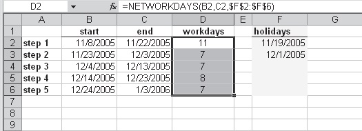
In this example a project has to be scheduled. Each of the five steps has a fixed start and end date. To determine the number of complete workdays between the start and end dates, the NETWORKDAYS function from the Analysis ToolPak add-in can be used. This function excludes weekends and any dates identified as non-workdays and holidays. The syntax is as follows:

NETWORKDAYS(start_date, end_date, holidays)

start_date: The start date.
end_date: The end date.
holidays: (optional) One or more dates that are to be excluded from the work schedule.

To determine the number of workdays:

1. In column B type the start date of each step.
2. In column C type the end date of each step.
3. List additional holidays in cells F2:F6.
4. Select cells D2:D6 and type the following formula:
=NETWORKDAYS(B2,C2,$F$2:$F$6).
5. Press <-Ctrl+Enter->.

Use the NETWORKDAYS function to determine the number of workdays

Use the WORKDAY function to calculate workdays - Date and Time Functions - Microsoft Excel Tutorials

Use the WORKDAY function to calculate workdays using Microsoft Excel

A worksheet is used to schedule a project. The project contains the start date and five major steps. Each step takes an estimated number of days to accomplish. To determine the correct end date, weekends and additional days off have to be taken into consideration. To perform this task, use the WORKDAY function from the Analysis ToolPak add-in. This function returns a date that is the indicated number of workdays before or after a date. Workdays exclude weekends and any dates identified as holidays. The syntax is as follows:

WORKDAY(start_date, days, holidays)

start_date: The start date.
days: The total number of available days, not counting weekends and holidays, before or after start_date. Both positive and negative values are acceptable.
holidays: (optional) One or more dates that are to be excluded from the work schedule.


To determine the end date of a project:

1. In cell C2, enter the start date of the project.
2. In column B enter the estimated days to finish each step.
3. In cell D2 type the following formula:
=WORKDAY(C3,B3,$F$2:$F$8).
4. In cells F1:F8 additional holidays can be listed individually.
5. In cell C3 type the formula =D2+1.
6. Fill cells C3 and D2 down to C6 and D6.

Use the WORKDAY function to calculate workdays

Use the EDATE function to calculate months - Date and Time Functions - Microsoft Excel Tutorials

Use the EDATE function to calculate months using Microsoft Excel

If a few months have to be added to or subtracted from a date, the EDATE function is very useful. This function returns a serial number that represents the date that is the indicated number of months before or after a specified date (offset).

In this example, column A of a worksheet contains the start dates. In column B, enter the offset in months to be added or subtracted. The result should show up in column C.

To use EDATE and add or subtract a number of months to start dates:

1. Enter different start dates in column A.
2. Enter offset months in column B.
3. Select cells C2:C10 and type the following formula:
=EDATE(A2,B2).
4. Press <-Ctrl+Enter->.

Use the EDATE function to calculate months using Microsoft Excel

Note: To use the EDATE function, the Analysis ToolPak add-in has to be installed as described in the previous example.

Use the WEEKNUM function to determine the week number - Date and Time Functions - Microsoft Excel Tutorials

Use the WEEKNUM function to determine the week number using Microsoft Excel

To determine the week number of a particular date (a very common practice in Europe), load the Analysis ToolPak add-in, accessed by choosing Add-Ins... from the Tools menu.

Now the WEEKNUM function is available. This function returns a number that indicates where the week falls numerically within a year.

To determine the week number:

1. Type different dates of the year in cells A2:A10.
2. Select cells B2:B10 and type the following formula:
=WEEKNUM(A2).
3. Press <-Ctrl+Enter->.

Use the WEEKNUM function to determine the week number

Watch the Video Tutorial - https://www.youtube.com/watch?v=sfaAHm0qO4k

 

Use the WEEKDAY function to calculate with different hourly pay rates - Date and Time Functions - Microsoft Excel Tutorials

Use the WEEKDAY function to calculate with different hourly pay rates using Microsoft Excel

Many companies calculate payroll using hourly rates for each employee. The hourly rates depend on which days are worked, as work performed on the weekend often is paid at a higher rate than work performed Monday through Friday.

In this example, different hourly rates are defined based on which days are worked. Column A lists the dates, column B has the custom format DDD to show the day of the week, and column C lists the number of hours worked.

To calculate with different hourly pay rates:

1. In a worksheet, enter the data shown in columns A, B, and C in Figure.
2. Select cell F2 and enter 12.50 (hourly rate for Monday through Friday).
3. Select cell F5 and enter 18.50 (hourly rate for Saturday and Sunday).
4. Select cells D2:D10 and type the following formula:
=IF(OR(WEEKDAY(A2)=1,WEEKDAY(A2)=7),C2*$F$5,C2*$F$2).
5. Press <-Ctrl+Enter->.

Use the WEEKDAY function to calculate with different hourly pay rates

Watch the Video Tutorial - https://www.youtube.com/watch?v=3jg_beNL-LI

 

Use the DAYS360 function to calculate with a 360-day year - Date and Time Functions - Microsoft Excel Tutorials

Use the DAYS360 function to calculate with a 360-day year using Microsoft Excel

If there is an accounting system installed that is based on 12 30-day months, the DAYS360 function can be used. This function returns the number of days between two dates based on a 360-day year. Here is the syntax:

DAYS360(start_date, end_date, method)

start_date: The start date.
end_date: The end date.
method: A logical value that specifies which method to use (U.S. or European).

U.S. (NASD) method: Used if method is FALSE. If the starting date is the 31st of a month, it is considered to be the 30th of the same month. If the ending date is the 31st of a month and the starting date is earlier than the 30th of the month, the ending date is considered to be the first of the next month; otherwise, the ending date is considered to be the 30th of the same month. European method: Used if method is TRUE. Starting or ending dates on the 31st of a month are considered to be the 30th of the same month.

To calculate with 360-day years:

1. In a worksheet, copy the data in columns A and B from Figure.
2. Select cells C2:C10 and type the following formula:
=DAYS360(A2,B2,FALSE).
3. Press <-Ctrl+Enter->.

Use the DAYS360 function to calculate with a 360-day year using Microsoft Excel

Watch the Video Tutorial - https://www.youtube.com/watch?v=RNyLlDJdklI

Use the EOMONTH function to determine the last day of a month - Date and Time Functions - Microsoft Excel Tutorials

Use the EOMONTH function to determine the last day of a month using Microsoft Excel

To find the last day of a month, use the EOMONTH function (EOMONTH(start_date, offset_months)). This function returns the date of the last day of the month, offset_months from start_date. If the function is not available, load the Analysis ToolPak add-in. Select Add-Ins... from the Tools menu bar and select Analysis ToolPak.

To determine the last day of a month:

1. In cells A2:A10 enter some dates.
2. In cells B2:B10 enter the desired offset from the start date (positive or negative values).
3. Select cells C2:C10 and type the following formula:
=EOMONTH(A2,B2).
4. Press <-Ctrl+Enter->.

Use the EOMONTH function to determine the last day of a month

Watch the Video Tutorial - https://www.youtube.com/watch?v=2y9snQMbJPU

 

Use the DATE function to add months to a date - Date and Time Functions - Microsoft Excel Tutorials

Use the DATE function to add months to a date using Microsoft Excel

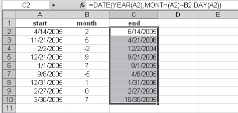
Let’s say we want to add a number of months to a given start date. In a new worksheet, list different start dates in column A. In column B, enter the number of months to be added to or subtracted from the start date. Based on that data, the end date can be calculated.

To add months to or subtract months from dates:

1. In cells A2:A10 list some start dates as shown in Figure.
2. List in cells B2:B10 the number of months to add or subtract.
3. Select cells C2:C10 and type the following formula:
=DATE(YEAR(A2),MONTH(A2)+B2,DAY(A2)).
4. Press <-Ctrl+Enter->.

Use the DATE function to add months to a date

Note: To determine an end date in the past, put a minus sign in front of the number of months.

Watch the Video Tutorial - https://www.youtube.com/watch?v=7eoIRTnVJ8M

 

Use the MONTH and DAY functions to sort birthdays by month - Date and Time Functions - Microsoft Excel Tutorials

Use the MONTH and DAY functions to sort birthdays by month using Microsoft Excel

The worksheet in Figure 4-14 contains a list of employees and their birthdays. This list has to be sorted by month, which is not possible with Excel’s usual sort function. Use this tip to insert a supporting column to convert the month and day dates to serial values.

To sort birthdays by month:

1. In cells A2:B10 generate a list of employees and their birthdays.
2. Select cells C2:C10 and type the following formula:
=MONTH(B2)*100+DAY(B2).
3. Press <-Ctrl+Enter->.
4. Select cell C1.
5. From the Standard toolbar, click Sort Ascending.
6. Format the column as General to display serial values rather than dates.

Use the MONTH and DAY functions to sort birthdays by month

Watch the Video Tutorial - https://www.youtube.com/watch?v=g9bFI1gEzOs

 

Use the DAY function to extract the day part of a date - Date and Time Functions - Microsoft Excel

Use the DAY function to extract the day part of a date using Microsoft Excel

Once again, use the worksheet from the previous two examples. Column A contains dates in different formats. To determine the day part of a date, use the DAY function. This function returns the day corresponding to a date as an integer in the range 1 to 31.

To extract the day as part of a date:

1. In cells A2:A10 generate a list of dates using different formats.
2. Select cells B2:B10 and type the following formula:
=DAY(A2).
3. Press <-Ctrl+Enter->.

Use the DAY function to extract the day part of a date

Note: If the day part is missing (see rows 5 and 6), the function returns the value 1.

Watch the Video Tutorial - https://www.youtube.com/watch?v=dQaRsEH7ZS8

 

Use the MONTH function to extract the month part of a date - Date and Time Functions - Microsoft Excel Tutorials

Use the MONTH function to extract the month part of a date using Microsoft Excel

For this tip use the worksheet from the previous example. Column A contains dates formatted in different ways. To determine the month part of a date, use the MONTH function. This function returns the month corresponding to a date as an integer in the range 1 to 12.

To extract the month part of a date:

1. In cells A2:A10 generate a list of dates using different formats.
2. Select cells B2:B10 and type the following formula:
=MONTH(A2).
3. Press <-Ctrl+Enter->.

Use the MONTH function to extract the month part of a date

Watch the Video Tutorial - https://www.youtube.com/watch?v=JAG3zRuYajU

 

Use the YEAR function to extract the year part of a date - Date and Time Functions - Microsoft Excel

Use the YEAR function to extract the year part of a date using Microsoft Excel

As shown in Figure, column A of a worksheet contains a list of dates formatted in different ways. To determine the year corresponding to a date, use the YEAR function. This function returns the year as an integer in the range 1900 to 9999. If the year is not specified, as in cell A9, the year is assumed to be the current year.

To extract the year as part of a date:

1. In cells A2:A10, generate a list of dates using different formats.
2. Select cells B2:B10 and type the following formula:
=YEAR(A2).
3. Press <-Ctrl+Enter->.

Use the YEAR function to extract the year part of a date

Watch the Video Tutorial - https://www.youtube.com/watch?v=IsJFpZD4yu0

Use the DATEVALUE function to recalculate dates formatted as text - Date and Time Functions - Microsoft Excel Tutorials

Use the DATEVALUE function to recalculate dates formatted as text using Microsoft Excel

Figure shows start and end dates in columns A and B. Excel cannot interpret the columns as dates because they are formatted as text. To convert and calculate these types of dates, use the DATEVALUE function. This function returns the serial number of the date represented by the “text date.”

Let’s determine the difference between start and end dates.

To calculate the difference between text dates:

1. Select cells C2:C10.
2. Type the following formula:
=DATEVALUE(B2)-DATEVALUE(A2).
3. Press <-Ctrl+Enter->.

Use the DATEVALUE function to recalculate dates formatted as text

Watch the Video Tutorial - https://www.youtube.com/watch?v=TGl_Ea0C5Wc