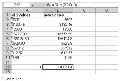
A worksheet contains values in column A that cannot be summed up because the first character in each cell is an apostrophe. How do you solve this problem? Use the SUBSTITUTE formula to replace specific characters in text or a cell.
SUBSTITUTE(text, old_text, new_text, instance_num)
text: The text or the reference to a cell containing text in which characters are substituted.
old_text: Text that should be replaced.new_text: Text that replaces old_text.
instance_num: Specifies which instance of old_text is to be replaced by new_text. If omitted, every instance of old_text is replaced.
1. Format column A as text.
2. Enter a series of numbers in cells A2:A10. Notice that Excel tags them with green triangles in the upper-left
corner to indicate the numbers have been entered as text.
3. Select cells B2:B10 and type the following formula: =VALUE(SUBSTITUTE(A2,"'","")).
4. Press <-Ctrl+Enter->.
5. Select cell A12, type the following formula: =SUM(A2:A10), and press <-Enter->.
6. Select cell B12, type the following formula: =SUM(B2:B10), and press <-Enter->.

Watch the Video Tutorial - https://www.youtube.com/watch?v=aJrW9TRugas
Hope You Like This Tutorial - Give Comments
I have to say that you guys are doing excellent work. Before reading your blog I wasn't aware that SUBSTITUTE functions can be used to substitute to many things such as characters, numbers etc. The method of substitution is very easy.
ReplyDeletedigital certificates